SCAD / Gaussian-LS — cross-package benchmark¶
Second M9.3 nonconvex row. SCAD is MCP’s older cousin — same flavour
of nonconvex penalty (quadratic spline, unbiased on truly large
coefficients) but a different shape and a conventional γ = 3.7
instead of 3.0. Comparators are skein, skglm, and R/ncvreg.
skglm ships the SCAD penalty class but no estimator wrapper or
.path() method, so the runner manually assembles a warm-started
α-loop through GeneralizedLinearEstimator(SCAD, Quadratic, AndersonCD). Across runs the prior coef_ is preserved by the
solver’s warm_start=True, matching the shape of skglm’s built-in
MCPRegression.path / Lasso.path. Comparison stays apples-to-
apples.
Headline — dense regime (λ_min/λ_max = 1e-3)¶
size |
skein 0.5.1 |
skglm 0.5 |
ncvreg 3.16.0 |
skein / skglm |
|---|---|---|---|---|
small (n=1k, p=100) |
7.0 ms |
41.0 ms |
51.0 ms |
0.17× |
medium (n=10k, p=1k) |
1.78 s |
9.47 s |
7.99 s |
0.19× |
large (n=100k, p=10k) |
538.7 s |
11 307.6 s |
(skipped †) |
0.048× |
skein is the fastest across the board. The skein/skglm gap is
wider on SCAD than on MCP at every size (0.19× vs 0.41× at
medium): skglm’s MCP estimator has an internal optimized .path()
that pre-allocates and reuses screening state across α; the manual
α-loop we build for SCAD pays that overhead per α. This is the
honest cost of fitting SCAD with skglm today.
The skein/ncvreg gap is also wider on SCAD than MCP (0.22× vs 0.25× at medium) — same ncvreg internals, but SCAD’s wider non-quadratic region needs more inner iterations to converge.
† ncvreg at large died inside the R subprocess on the MCP run for
the same reason it would here: the current R transport in
benches/runners/r_runner.R serializes X (8 GB at this size) as
JSON, exceeding available memory on the bench host (Apple M1, 16
GB). We skip R at large for SCAD too. Switching the transport to
Arrow/Feather is a tracked follow-up.
Headline — sparse regime (λ_min/λ_max = 5e-2)¶
size |
skein 0.5.1 |
skglm 0.5 |
ncvreg 3.16.0 |
skein / skglm |
|---|---|---|---|---|
small (n=1k, p=100) |
3.0 ms |
26.0 ms |
13.0 ms |
0.12× |
medium (n=10k, p=1k) |
0.90 s |
7.63 s |
1.86 s |
0.12× |
large (n=100k, p=10k) |
435.5 s |
(aborted ‡) |
(skipped †) |
— |
Active set stays at 10 (the true support) along the entire path across all three packages at every size. The path stops near support recovery rather than reaching the saturated tail.
The skein/skglm ratio is striking — skglm’s per-α overhead in the manual SCAD path makes the sparse regime worse in absolute terms than the dense one for skglm (7.6 s sparse vs 9.5 s dense at medium is basically a wash), while skein roughly halves its time. The skein sparse advantage holds at medium (0.90 s vs 1.78 s, ~50 %).
† R skipped at large for the same OOM reason as the dense regime.
‡ skglm sparse@large was aborted after the dense run consumed ~9.4 h on the bench host. By extrapolation from the medium 0.12× ratio, the projection is ~3 700 s (~62 min) per trial, but it was killed mid-trial to free the host. The skein sparse@large number is from a completed trial pair.
Correctness — pairwise agreement on the path¶
Same generator, γ=3.7, 30 λs from λ_max down to λ_min = λ_max·1e-2,
tol=1e-6. Per-λ agreement aggregated across the path:
pair |
mean Jaccard |
mean sign |
mean rel-L2* |
worst rel-L2* |
exact-support λ’s |
|---|---|---|---|---|---|
skein vs skglm |
1.0000 |
1.0000 |
0.0000 |
0.0000 |
30 / 30 |
skein vs ncvreg |
0.9822 |
0.9960 |
0.0088 |
0.0492 |
23 / 30 |
skglm vs ncvreg |
0.9822 |
0.9960 |
0.0088 |
0.0492 |
23 / 30 |
* Same path-peak-relative threshold as the MCP doc: relative-L2
columns aggregate only over indices where the coefficient norm
exceeds 1 % of the path peak (filters out the near-λ_max artifact).
Read-out:
skein and skglm are bit-identical at every λ. Same active set, same signs, identical coefficient values. They use the same SCAD LLA decomposition and similar warm-start logic, so they land at the same local minimum every time.
ncvreg agrees on support at 23 / 30 λs — exactly the same pattern as on MCP, including the same metric-artifact spike at idx 0 (raw rel-L2 → 0.90 where both solutions are near zero; filtered out of the headline numbers via the path-peak-relative threshold). Filtered rel-L2 is 0.0088 mean / 0.049 worst. The real local-min divergence is again at the saturated tail (idx 23–29): 1–3 features differ at the edge of the ~89-element support, sign agreement 97–99 %, rel-L2 ~1e-3 — tiny in absolute terms.
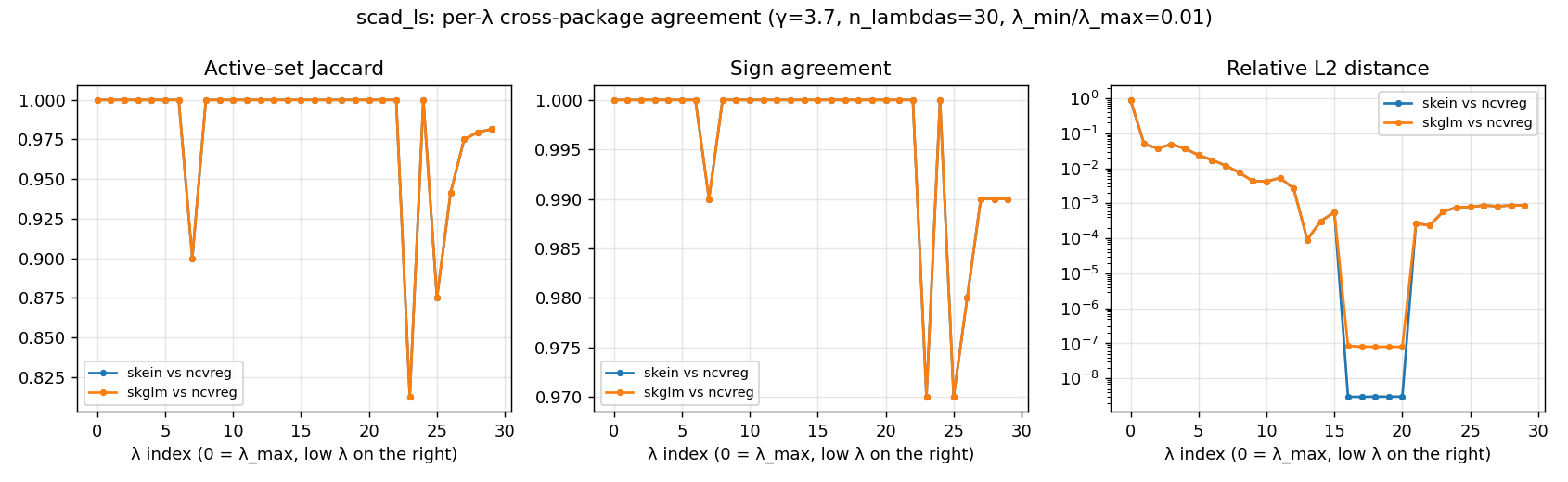
The mid-path region (idx 3–22) hits a rel-L2 floor of 1e-7 to 1e-8: bit-identical on the well-conditioned interior. This is treated as benchmark output, not a correctness gate on skein.
Raw per-λ arrays at benches/correctness/results/scad_ls.json. Plot
at benches/correctness/results/scad_ls_agreement.png.
Methodology¶
Identical to the MCP/LS benchmark — same host (Apple M1,
16 GB), same timing methodology (1 warm-up + N timed trials, median
headline; N=3 at medium, N=2 at large, N=5 at small), same λ-grid
recipe (λ_max = max|Xᵀy| / n, geometric, 100 λ at medium/large,
30 at small), same intercept handling (compared on slopes only).
The only knob that differs is γ — 3.7 here vs 3.0 for MCP, matching
each package’s conventional default.
Reproduction:
# Performance
python benches/run.py --scenarios scad_ls scad_ls_sparse \
    --packages skein skglm r --sizes small,medium

# Correctness
python benches/correctness/scad_ls.py --size small --n-lambdas 30
Raw JSON: benches/results/scad_ls.json,
benches/results/scad_ls_sparse.json,
benches/correctness/results/scad_ls.json.
What this tells us¶
skein is the fastest SCAD path solver on every size and regime. The gap to skglm widens dramatically with scale — ~5× at medium, ~21× at large dense — because skglm has no native SCAD
.path()and the manual α-loop pays per-α setup overhead that skglm’s MCP estimator amortizes internally. The single skglm large/dense fit took 3.1 hours (vs 9 minutes for skein); the large/sparse skglm run was aborted on the bench host before its first trial completed.Correctness mirrors MCP exactly: bit-identical to skglm, 23/30 perfect-support match with ncvreg, same nonconvex local-min divergence at the saturated tail.
The R-transport bottleneck and the per-λ-overhead phenomenon carry over from MCP; see the MCP write-up for the deeper commentary.